This example has been auto-generated from the examples/ folder at GitHub repository.

Gaussian Mixture

# Activate local environment, see `Project.toml`
import Pkg; Pkg.activate(".."); Pkg.instantiate();

This notebook illustrates how to use the NormalMixture node in RxInfer.jl for both univariate and multivariate observations.

Load packages

using RxInfer, Plots, Random, LinearAlgebra, StableRNGs, LaTeXStrings

Univariate Gaussian Mixture Model

Consider the data set of length $N$ observed below.

function generate_univariate_data(nr_samples; rng = MersenneTwister(123))

    # data generating parameters
    class        = [1/3, 2/3]
    mean1, mean2 = -10, 10
    precision    = 1.777

    # generate data
    z = rand(rng, Categorical(class), nr_samples)
    y = zeros(nr_samples)
    for k in 1:nr_samples
        y[k] = rand(rng, Normal(z[k] == 1 ? mean1 : mean2, 1/sqrt(precision)))
    end

    return y

end;

data_univariate = generate_univariate_data(100)
histogram(data_univariate, bins=50, label="data", normed=true)
xlims!(minimum(data_univariate), maximum(data_univariate))
ylims!(0, Inf)
ylabel!("relative occurrence [%]")
xlabel!("y")

Model specification

The goal here is to create a model for the data set above. In this case a Gaussian mixture model with $K$ components seems to suite the situation well. We specify the factorized model as $p(y, z, s, m, w) = \prod_{n=1}^N \bigg(p(y_n \mid m, w, z_n) p(z_n \mid s) \bigg)\prod_{k=1}^K \bigg(p(m_k) p(w_k) \bigg) p(s),$ where the individual terms are specified as $\begin{aligned} p(s) &= \mathrm{Beta}(s \mid \alpha_s, \beta_s) \\ p(m_{k}) &= \mathcal{N}(m_k \mid \mu_k, \sigma_k^2) \\ p(w_{k}) &= \Gamma(w_k \mid \alpha_k, \beta_k) \\ p(z_n \mid s) &= \mathrm{Ber}(z_n \mid s) \\ p(y_n \mid m, w, z_n) &= \prod_{k=1}^K \mathcal{N}\left(y_n \mid m_{k}, w_{k}\right)^{z_{nk}} \end{aligned}$

The set of observations $y = \{y_1, y_2, \ldots, y_N\}$ is modeled by a mixture of Gaussian distributions, parameterized by means $m = \{m_1, m_2, \ldots, m_K\}$ and precisions $w = \{ w_1, w_2, \ldots, w_K\}$, where $k$ denotes the component index. This component is selected per observation by the indicator variable $z_n$, which is a one-of-$K$ encoded vector satisfying $\sum_{k=1}^K z_{nk} = 1$ and $z_{nk} \in \{0, 1\} \forall k$. We put a hyperprior on these variables, termed $s$, which represents the relative occurrence of the different realizations of $z_n$.

Here we implement the following model with uninformative values for the hyperparameters as

@model function univariate_gaussian_mixture_model(y)
    
    s ~ Beta(1.0, 1.0)

    m[1] ~ Normal(mean = -2.0, variance = 1e3)
    w[1] ~ Gamma(shape = 0.01, rate = 0.01)

    m[2] ~ Normal(mean = 2.0, variance = 1e3)
    w[2] ~ Gamma(shape = 0.01, rate = 0.01)

    for i in eachindex(y)
        z[i] ~ Bernoulli(s)
        y[i] ~ NormalMixture(switch = z[i], m = m, p = w)
    end
    
end

Probabilistic inference

In order to fit the model to the data, we are interested in computing the posterior distribution $p(z, s, m, w \mid y)$ However, computation of this term is intractable. Therefore, it is approximated by a naive mean-field approximation, specified as $p(z, s, m, w \mid y) \approx \prod_{n=1}^N q(z_n) \prod_{k=1}^K \bigg(q(m_k) q(w_k)\bigg) q(s),$ with the functional forms $\begin{aligned} q(s) &= \mathrm{Beta}(s \mid \hat{\alpha}_s, \hat{\beta}_s) \\ q(m_k) &= \mathcal{N}(m_k \mid \hat{\mu}_k, \hat{\sigma}^2_k) \\ q(w_k) &= \Gamma (w_k \mid \hat{\alpha}_k, \hat{\beta}_k) \\ q(z_n) &= \mathrm{Ber}(z_n \mid \hat{p}_n) \end{aligned}$ In order to get the inference procedure started, these marginal distribution need to be initialized.

n_iterations = 10

init = @initialization begin
    q(s) = vague(Beta)
    q(m) = [NormalMeanVariance(-2.0, 1e3), NormalMeanVariance(2.0, 1e3)]
    q(w) = [vague(GammaShapeRate), vague(GammaShapeRate)]
end

results_univariate = infer(
    model = univariate_gaussian_mixture_model(), 
    constraints = MeanField(),
    data  = (y = data_univariate,), 
    initialization = init, 
    iterations  = n_iterations, 
    free_energy = true
)

Inference results:
  Posteriors       | available for (m, w, s, z)
  Free Energy:     | Real[245.113, 188.579, 149.369, 121.985, 121.592, 121.
591, 121.591, 121.591, 121.591, 121.591]

Results

Below the inference results can be seen as a function of the iterations

m1 = [results_univariate.posteriors[:m][i][1] for i in 1:n_iterations]
m2 = [results_univariate.posteriors[:m][i][2] for i in 1:n_iterations]
w1 = [results_univariate.posteriors[:w][i][1] for i in 1:n_iterations]
w2 = [results_univariate.posteriors[:w][i][2] for i in 1:n_iterations];

mp = plot(mean.(m1), ribbon = std.(m1) .|> sqrt, label = L"posterior $m_1$")
mp = plot!(mean.(m2), ribbon = std.(m2) .|> sqrt, label = L"posterior $m_2$")
mp = plot!(mp, [ -10 ], seriestype = :hline, label = L"true $m_1$")
mp = plot!(mp, [ 10 ], seriestype = :hline, label = L"true $m_2$")

wp = plot(mean.(w1), ribbon = std.(w1) .|> sqrt, label = L"posterior $w_1$", legend = :bottomright, ylim = (-1, 3))
wp = plot!(wp, mean.(w2), ribbon = std.(w2) .|> sqrt, label = L"posterior $w_2$")
wp = plot!(wp, [ 1.777 ], seriestype = :hline, label = L"true $w_1$")
wp = plot!(wp, [ 1.777 ], seriestype = :hline, label = L"true $w_2$")

swp = plot(mean.(results_univariate.posteriors[:s]), ribbon = std.(results_univariate.posteriors[:s]) .|> sqrt, label = L"posterior $s$")
swp = plot!(swp, [ 2/3 ], seriestype = :hline, label = L"true $s$")

fep = plot(results_univariate.free_energy, label = "Free Energy", legend = :topright)

plot(mp, wp, swp, fep, layout = @layout([ a b; c d ]), size = (800, 400))
xlabel!("iteration")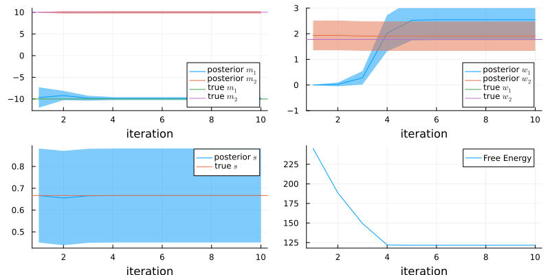

Multivariate Gaussian Mixture Model

The above example can also be extended to the multivariate case. Consider the data set below

function generate_multivariate_data(nr_samples; rng = MersenneTwister(123))

    L         = 50.0
    nr_mixtures = 6

    probvec = normalize!(ones(nr_mixtures), 1)

    switch = Categorical(probvec)

    gaussians = map(1:nr_mixtures) do index
        angle      = 2π / nr_mixtures * (index - 1)
        basis_v    = L * [ 1.0, 0.0 ]
        R          = [ cos(angle) -sin(angle); sin(angle) cos(angle) ]
        mean       = R * basis_v 
        covariance = Matrix(Hermitian(R * [ 10.0 0.0; 0.0 20.0 ] * transpose(R)))
        return MvNormal(mean, covariance)
    end

    z = rand(rng, switch, nr_samples)
    y = Vector{Vector{Float64}}(undef, nr_samples)

    for n in 1:nr_samples
        y[n] = rand(rng, gaussians[z[n]])
    end

    return y

end;

data_multivariate = generate_multivariate_data(500)

sdim(n) = (a) -> map(d -> d[n], a) # helper function
scatter(data_multivariate |> sdim(1), data_multivariate |> sdim(2), ms = 2, alpha = 0.4, size = (600, 400), legend=false)
xlabel!(L"y_1")
ylabel!(L"y_2")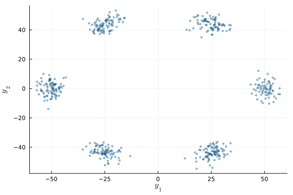

Model specification

The goal here is to create a model for the data set above. In this case a Gaussian mixture model with $K$ components seems to suite the situation well. We specify the factorized model as $p(y, z, s, m, w) = \prod_{n=1}^N \bigg(p(y_n \mid m, W, z_n) p(z_n \mid s) \bigg)\prod_{k=1}^K \bigg(p(m_k) p(W_k) \bigg) p(s),$ where the individual terms are specified as $\begin{aligned} p(s) &= \mathrm{Dir}(s \mid \alpha_s) \\ p(m_{k}) &= \mathcal{N}(m_k \mid \mu_k, \Sigma_k) \\ p(W_{k}) &= \mathcal{W}(W_k \mid V_k, \nu_k) \\ p(z_n \mid s) &= \mathrm{Cat}(z_n \mid s) \\ p(y_n \mid m, W, z_n) &= \prod_{k=1}^K \mathcal{N}\left(y_n \mid m_{k}, W_{k}\right)^{z_{nk}} \end{aligned}$

The set of observations $y = \{y_1, y_2, \ldots, y_N\}$ is modeled by a mixture of Gaussian distributions, parameterized by means $m = \{m_1, m_2, \ldots, m_K\}$ and precisions $W = \{ W_1, W_2, \ldots, W_K\}$, where $k$ denotes the component index. This component is selected per observation by the indicator variable $z_n$, which is a one-of-$K$ encoded vector satisfying $\sum_{k=1}^K z_{nk} = 1$ and $z_{nk} \in \{0, 1\} \forall k$. We put a hyperprior on these variables, termed $s$, which represents the relative occurrence of the different realizations of $z_n$.

@model function multivariate_gaussian_mixture_model(nr_mixtures, priors, y)
    local m
    local w

    for k in 1:nr_mixtures        
        m[k] ~ priors[k]
        w[k] ~ Wishart(3, 1e2*diagm(ones(2)))
    end
    
    s ~ Dirichlet(ones(nr_mixtures))
    
    for n in eachindex(y)
        z[n] ~ Categorical(s) 
        y[n] ~ NormalMixture(switch = z[n], m = m, p = w)
    end
    
end

Probabilistic inference

In order to fit the model to the data, we are interested in computing the posterior distribution $p(z, s, m, W \mid y)$ However, computation of this term is intractable. Therefore, it is approximated by a naive mean-field approximation, specified as $p(z, s, m, W \mid y) \approx \prod_{n=1}^N q(z_n) \prod_{k=1}^K \bigg(q(m_k) q(W_k)\bigg) q(s),$ with the functional forms $\begin{aligned} q(s) &= \mathrm{Dir}(s \mid \hat{\alpha}_s) \\ q(m_k) &= \mathcal{N}(m_k \mid \hat{\mu}_k, \hat{\Sigma}_k) \\ q(w_k) &= \mathcal{W}(W_k \mid \hat{V}_k, \hat{\nu}_k) \\ q(z_n) &= \mathrm{Cat}(z_n \mid \hat{p}_n) \end{aligned}$ In order to get the inference procedure started, these marginal distribution need to be initialized.

rng = MersenneTwister(121)
priors = [MvNormal([cos(k*2π/6), sin(k*2π/6)], diagm(1e2 * ones(2))) for k in 1:6]
init = @initialization begin
    q(s) = vague(Dirichlet, 6)
    q(m) = priors
    q(w) = Wishart(3, diagm(1e2 * ones(2)))
end

results_multivariate = infer(
    model = multivariate_gaussian_mixture_model(
        nr_mixtures = 6, 
        priors = priors,
    ), 
    data  = (y = data_multivariate,), 
    constraints   = MeanField(),
    initialization = init, 
    iterations  = 50, 
    free_energy = true
)

Inference results:
  Posteriors       | available for (w, m, s, z)
  Free Energy:     | Real[3946.64, 3902.88, 3902.88, 3902.88, 3902.88, 3902
.88, 3902.88, 3902.88, 3902.88, 3902.88  …  3902.88, 3902.88, 3902.88, 3902
.88, 3902.88, 3902.88, 3902.88, 3902.88, 3902.88, 3902.88]

Results

Below the inference results can be seen

p_data = scatter(data_multivariate |> sdim(1), data_multivariate |> sdim(2), ms = 2, alpha = 0.4, legend=false, title="Data", xlims=(-75, 75), ylims=(-75, 75))
p_result = plot(xlims = (-75, 75), ylims = (-75, 75), title="Inference result", legend=false, colorbar = false)
for (e_m, e_w) in zip(results_multivariate.posteriors[:m][end], results_multivariate.posteriors[:w][end])
    gaussian = MvNormal(mean(e_m), Matrix(Hermitian(mean(inv, e_w))))
    global p_result = contour!(p_result, range(-75, 75, step = 0.25), range(-75, 75, step = 0.25), (x, y) -> pdf(gaussian, [ x, y ]), title="Inference result", legend=false, levels = 7, colorbar = false)
end
p_fe = plot(results_multivariate.free_energy, label = "Free Energy")

plot(p_data, p_result, p_fe, layout = @layout([ a b; c ]))